Cocktail Party Problem

Imagine being in a party. Like in every party, the music is loud and everyone is screaming. Nevertheless, you can hear (almost) clearly the person that you are talking with. This capacity to focus your attention on a conversation in a noisy environment is what the psychoacousticians call the cocktail party effect. This effect becomes a problem when the person is unable to focus its attention on a particular stimulus. The cocktail party problem has first been studied in the early 1950s in the context of air traffic controls. Since then, this problem grew beyond the realm of psychology and we can use computational methods to solve it.
Here, we are going to present the most commonly used approach, named Independent Component Analysis (ICA), through the implementation of the FastICA algorithm.

ICA

To solve the cocktail party problem, we have to isolate the sounds coming from the different sources. More formally, we have to separate multivariate signals into multiple independent signals. When using ICA, we are looking for independent components that will maximize the statistical independence of the estimated components. So, how can we force the estimated components to be as independent as possible ?

There are two approaches: we can try to minimize the mutual information of the components or, we can try to maximize the non-Gaussianity of the components. Here, we are going to focus on the second approach as it is the one used in FastICA.
Non-Gaussianity can be defined as a high/low level of spikiness of a distribution (here represented by an audio signal). The degree of spikiness of a distribution can be measured by using the normalized form of the fourth central moment of the distribution, also called Kurtosis. It is defined by this formula:

$kurtosis(x) = \mathop{\mathbb{E}}\{{x}^{4}\} - 3{(\mathop{\mathbb{E}}\{{x}^{2}\})}^{2}$

If we assume that $x$ is a zero mean and unit variance variable, kurtosis becomes:

$kurtosis(x) = \mathop{\mathbb{E}}\{{x}^{4}\} - 3$

Kurtosis measure is positive if the distribution is spikier than Gaussian and negative if it is flatter. The non-Gaussianity can therefore be measured by computing the absolute value of the Kurtosis measure.

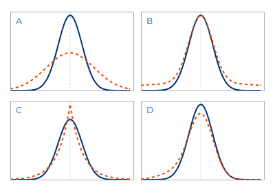
*Gaussian distribution (blue) compared to distribution with different Kurtosis measure (red)*

However, this measure is extremely sensitive to outliers and is not a robust way to determine the non-Gaussianity of a distribution.
According to the Central Limit Theorem[1], when independent random variables are added, their normalized sum tends toward a Gaussian distribution. We can use this theorem to define the Gaussianity of a distribution in terms of entropy, the distribution with the highest entropy being the Gaussian distribution. The entropy of a random variable $y$ with the density function $p(y)$ is defined as follow:

$H(y) = -\mathop{\mathbb{E}}\{\log{p_{i}(y)}\}$

Based on the property of the Gaussian distribution in terms of entropy and on the above definition of the entropy, we can define the negentropy as follow:

$J(y) = H(y_{G}) - H(y)$

where $y_{G}$ is a Gaussian variable with the same variance as $y$ .
Gaussian distribution being the distribution with the highest entropy, $H(y_{G})$ > $H(y)$ with the assumption that $y$ is not Gaussian (which is the case in the cocktail party problem). Therefore, to find the most non-Gaussian $y$ we have to maximize $J(y)$ . However, in practice we can’t directly maximize the negentropy as it is computationally expensive. Instead, we try to maximize an approximation of the negentropy. The negentropy approximation used by FastICA is the following:

$J(y) \approx [\mathop{\mathbb{E}}\{G(y)\} - \mathop{\mathbb{E}}\{G(g)\}]^2$

where $G$ is a non-quadratic function, $y$ a zero mean and unit variance variable and $g$ a Gaussian zero mean and unit variance variable. In the case of FastICA, $G(x) = \log\cosh(x)$ .
Moreover, since $\mathop{\mathbb{E}}\{G(g)\}$ is contant, we just have to maximize $\mathop{\mathbb{E}}\{G(y)\}$ in order to maximize $J(y)$ . That’s where FastICA comes into play !

FastICA

Let $X$ be the input data matrix of size $N$ x $M$ , $w$ a weight vector of size $N$ and $C$ the number of components. We want to find the matrix $W$ of size $N$ x $C$ that will project $X$ onto independent component (i.e. $W^{T}X =$ matrix with independent components).

For FastICA to work we need to make sure that $\mathop{\mathbb{E}}\{XX^{T}\} = I$ . We accomplish this by centering and whitening the input data matrix $X$ . To center $X$ , we subtract to each of its column the mean value of the column:

$x_{ij} = x_{ij} - \frac{1}{M}\sum_{k}x_{ik}$

To whiten $X$ , we perform an eigenvalue decomposition on the covariance matrix of the centered $X$ :

$X = D^{\frac{-1}{2}}E^{T}X$

where $D$ is the diagonal matrix of eigenvalues and $E$ the matrix of eigenvectors.

In this setting we have:

$y = w^{T}X$

$J(w^{T}X) \approx [\mathop{\mathbb{E}}\{G(w^{T}X)\} - \mathop{\mathbb{E}}\{G(g)\}]^2$

The problem is now to find the unit vector $w$ so that $w^{T}X$ maximizes the non-Gaussianity. We can achieve that by using an approximative iteration of Newton’s Method defined by:

$w_{p} = w_{p} - \frac{J'(w_{p}^{T}X)}{J''(w_{p}^{T}X)}$

To do so, we have to compute the gradient and the derivative of the gradient of $J(w_{p}^{T}X)$ according to $w_{p}$ . We have:

$J'(w_{p}^{T}X) \propto \mathop{\mathbb{E}}\{XG'(w_{p}^{T}X)\}$

$J''(w_{p}^{T}X) \propto \mathop{\mathbb{E}}\{XX^{T}G''(w_{p}^{T}X)\}$

For the reasons explained on page 188 of [2], we cannot use directly this gradient. We have to add $w_{p}$ multiplied by a constant $\alpha$ . We obtain:

$J'(w_{p}^{T}X) \propto \mathop{\mathbb{E}}\{XG'(w_{p}^{T}X)\} + \alpha w_{p}$

$J''(w_{p}^{T}X) \propto \mathop{\mathbb{E}}\{XX^{T}G''(w_{p}^{T}X)\} + \alpha I$

The approximative Newton’s iteration becomes:

$w_{p} = w_{p} - \frac{\mathop{\mathbb{E}}\{XG'(w_{p}^{T}X)\} + \alpha w_{p}}{\mathop{\mathbb{E}}\{XX^{T}G''(w_{p}^{T}X)\} + \alpha I}$

With the assumption that $X$ has been centered and whitened and that $\mathop{\mathbb{E}}\{XX^{T}G''(w_{p}^{T}X)\} \approx \mathop{\mathbb{E}}\{XX^{T}\}\mathop{\mathbb{E}}\{G''(w_{p}^{T}X)\}$ , it can be simplified to:

$w_{p} = \mathop{\mathbb{E}}\{XG'(w_{p}^{T}X)\} - \mathop{\mathbb{E}}\{G''(w_{p}^{T}X)\}w_{p}$

We now have a one-unit algorithm to solve the cocktail party problem. But, we don’t want to estimate only one independent component but multiple ones. A method, is to add after the Newton’s iteration a deflationary orthogonalization step defined by:

$w_{p} = w_{p} - \sum_{i=1}^{p-1}(w_{p}^{T}w_{i})w_{i}$

More details can be found on page 192-194 of [2].

Algorithm

The complete algorithm will then look like this:

Center the matrix $X$
Whiten the matrix $X$
Create a matrix $W$ that will contain all the $w_{p}$
Repeat steps C times
4.1 Create a random vector of weight $w_{p}$ of size $N$
4.2 Perform a newton iteration on $w_{p}$
4.3 Perform a deflationary orthogonalization on $w_{p}$ using the current $W$
4.4 Normalize $w_{p}$
4.5 If $w_{p}$ is still changing go back to step 4.2
4.6 Put $w_{p}$ in $W$
Compute and return $W^{T}X$

Implementation

The implementation of the above algorithm is straightforward using Python and the Numpy library.

import numpy as np


# Definition of G'
def Gprime(x):
    return np.tanh(x)

# Definition of G''
def Gsecond(x):
    return np.ones(x.shape) - np.power(np.tanh(x), 2)

# Center matrix X
def centerMatrix(X, N):
    mean = X.mean(axis=1)
    M = X - (mean.reshape((N, 1)) @ np.ones((1, X.shape[1])))
    return M

# Whiten matrix X with eigenvalue decomposition
def whitenMatrix(X):
    D, E = np.linalg.eigh(X @ X.T)
    DE = np.diag(1/np.sqrt(D + 1e-5)) @ E.T
    
    return DE @ X

# One-unit algorithm step
def oneUnit(X, wp):
    term1 = np.mean((X @ Gprime(wp @ X).T), axis=1)
    term2 = np.mean(Gsecond(wp @ X), axis=1) * wp
    return term1 - term2

# Deflationary orthogonalization
def orthogonalize(W, wp, i):
    return wp - ((wp @ W[:i,:].T) @ W[:i,:])

# wp normalization
def normalize(wp):
    return wp / np.linalg.norm(wp)


def fastICA(X, C, max_iter):
    N = X.shape[0]
    X = centerMatrix(X, N)
    X = whitenMatrix(X)
    
    W = np.zeros((C, N))
    for i in range(C):
        wp = np.random.rand(1, N)
        for _ in range(max_iter):
            wp = oneUnit(X, wp)
            wp = orthogonalize(W, wp, i)
            wp = normalize(wp)
            W[i,:] = wp

    return W @ X

Results

Let’s now load some audio samples and see the results. Here we are going to use a dataset containing sounds coming from 9 different sources. You can find the data, the complete code and the results on my github.

from scipy.io import wavfile
import matplotlib.pyplot as plt
import numpy as np
import os

# Function to load the audio data
def loadData(dataPath, nsources=9, size=50000):
    data = np.empty((nsources, size), np.float32)

    for i in range(nsources):
        fs, data[i,:] = wavfile.read(os.path.join(dataPath, 'mix') + str(i+1) + '.wav')

    return fs, data

# Function to display the audio spectrum
def displayData(X):
    C = X.shape[0]

    for i in range(C):
        plt.subplot(C, 1, i + 1)
        plt.plot(X[i,:])
    plt.show()

# Function to save the audio data separated by fastica
def saveData(saveDataPath, fs, X):
    for i in range(X.shape[0]):
        wavfile.write(os.path.join(saveDataPath, 'ica_') + str(i + 1) + ".wav", fs, X[i,:])


dataPath = ""  # path to the folder containing the mix audio sounds
saveDataPath = ""  # path to the folder that will contain the results of the fastICA
nComponents = 9  # number of components that we want

if not os.path.exists(saveDataPath):
    os.makedirs(saveDataPath)

fs, X = loadData(dataPath)
displayData(X)

S = fastICA(X, nComponents)
displayData(S)

saveData(saveDataPath, fs, S)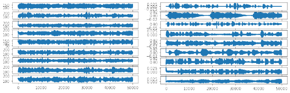

*Data matrix before (left) and after (right) FastICA*

References

[1] MIT OpenCourseWare on Central Limit Theorem and the Law of Large Numbers by Jeremy Orloff and Jonathan Bloom
[2] Independent Component Analysis by Aapo Hyvarinen, Juha Karhunen and Erkki Oja