Introduction
Human visual perception can be extremely limited compared to the rest of the animal kingdom. We see just a tiny part of the light spectrum and we can hardly perceive tiny movements thus missing potentially important information from our environment. In 2012, Hao-Yu Wu and his team published the paper Eulerian Video Magnification for Revealing Subtle Changes in the World containing a method that allows us to amplify colors and motions from a simple video to help us visualize imperceptible changes from the world around us. Here, we present this method and provide a simple implementation of the algorithm.
YIQ Color Space
The first step of the magnification algorithm is to convert RGB images composing the input video to YIQ. The Y component represents the brightness, I and Q represent the chrominance (i.e. the color information). This color space allows us to influence the colors of an image independently from its brightness. The conversion from RGB to YIQ can be done with the following formula:
$$\begin{bmatrix}Y \\ I \\ Q\end{bmatrix} = \begin{bmatrix}0.299 & 0.587 & 0.114 \\ 0.59590059 & -0.27455667 & -0.32134392 \\ 0.21153661 & -0.52273617 & 0.31119955\end{bmatrix}\begin{bmatrix}R \\ G \\ B\end{bmatrix}$$
Colors Magnification
Gaussian Pyramids
For the colors magnification we need to construct a Gaussian Pyramid of level \(l\) for each frame of the input video. This is done by taking the YIQ version of the original frame and downsampling it by a factor 2 for each new level of the pyramid.
The first step of the downsampling is to apply to the image a 2D Convolution with the following 5x5 Gaussian Kernel:
$$G_{k} = \frac{1}{256}\begin{bmatrix}1 & 4 & 6 & 4 & 1\\4 & 16 & 24 & 16 & 4\\6 & 24 & 36 & 24 & 6\\4 & 16 & 24 & 16 & 4\\1 & 4 & 6 & 4 & 1\end{bmatrix}$$
Once the convolution is done, we keep only 1 in 2 pixels in the rows and columns of the image giving us a downsampled image with height and width divided by 2 compared to the previous level of the pyramid. We do this process \(l - 1\) times.
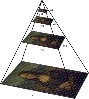
Gaussian Pyramid Levels Visualisation
Note that for the next steps of the colors magnification we keep only the last level of the pyramid. More precisely we will use the upsampled version of the last level of the pyramid. To obtain this upsampled image, we take the last level of the pyramid, add one pixel set to \(0\) every 2 pixels in the rows and columns of the downsampled image and apply \(4 \times G_{k}\). We obtain an image with height and width multiplied by 2 compared to the previously upsampled image. We do this process \(l - 1\) times i.e. until obtaining an upsampled image with the same dimension as the original image.
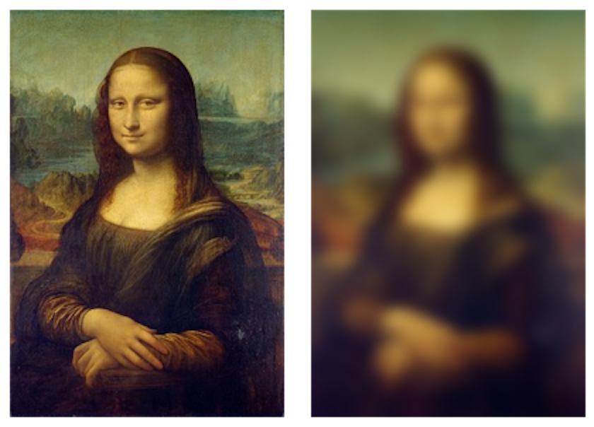
Original Image (left) and Upsampled Image from Gaussian Pyramid with \(l = 3\) (right)
Ideal Temporal Filter
The next and most important step is to filter the Gaussian Pyramid in order to keep only the pixels within our frequency band of interest \([\omega_{l}, \omega_{h}]\). For that, we need to switch from the spatial domain (our image) to the frequency domain using a Fourier Transform (see [2] for more details).
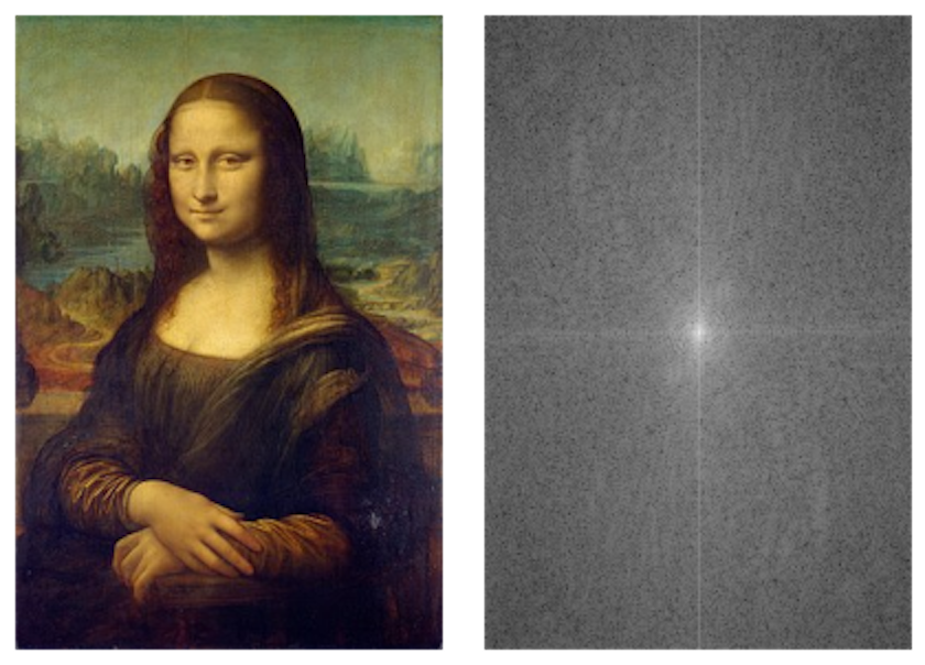
Original Image (left) and Its Magnitude Spectrum in the Frequency Domain (right)
In the frequency domain we keep only the frequencies withnin the \([\omega_{l}, \omega_{h}]\) range and set the other frequencies to \(0\). Then we can apply the Inverse Fourier Transform to retrieve a filtered image. Note that the result of an Inverse Fourier Transform is a matrix of complex numbers, we simply take the real part of each numbers of the complex matrix.
Below, you can see the result of an ideal temporal filter with \(\omega_{l} = 0.8333\) and \(\omega_{h} = 1\):
Image Magnification & Reconstruction
In order to magnify the colors obtained with the filtered pyramid \(F_{p}\) we introduce a value \(\alpha\) that will act as an amplification factor. To prevent the creation of artifacts in the output image we introduce another value \(A\) that will act as an attenuation factor for the chrominance components of the image. We obtain our magnified filtered pyramid \(M_{F_{p}}\) with attenuated chrominance with the following formula:
$$M_{F_{p}} = \begin{cases}\alpha F_{p}\ \text{if Y component}\\ \alpha A F_{p}\ \text{if I or Q component}\end{cases}$$
Finally, we reconstruct our image by adding \(M_{F_{p}}\) to the YIQ version of the original image, converting the resulting image to RGB and limiting the values of the resulting RGB image to \([0, 255]\) for each components. We repeat the previous process for each frame of the video.
Motions Magnification
Laplacian Pyramids
For the motions magnification, we want to focus on the edges of the objects in the video. To do so, we use the difference between two adjacent levels of the Gaussian Pyramid i.e. a Laplacian Pyramid.
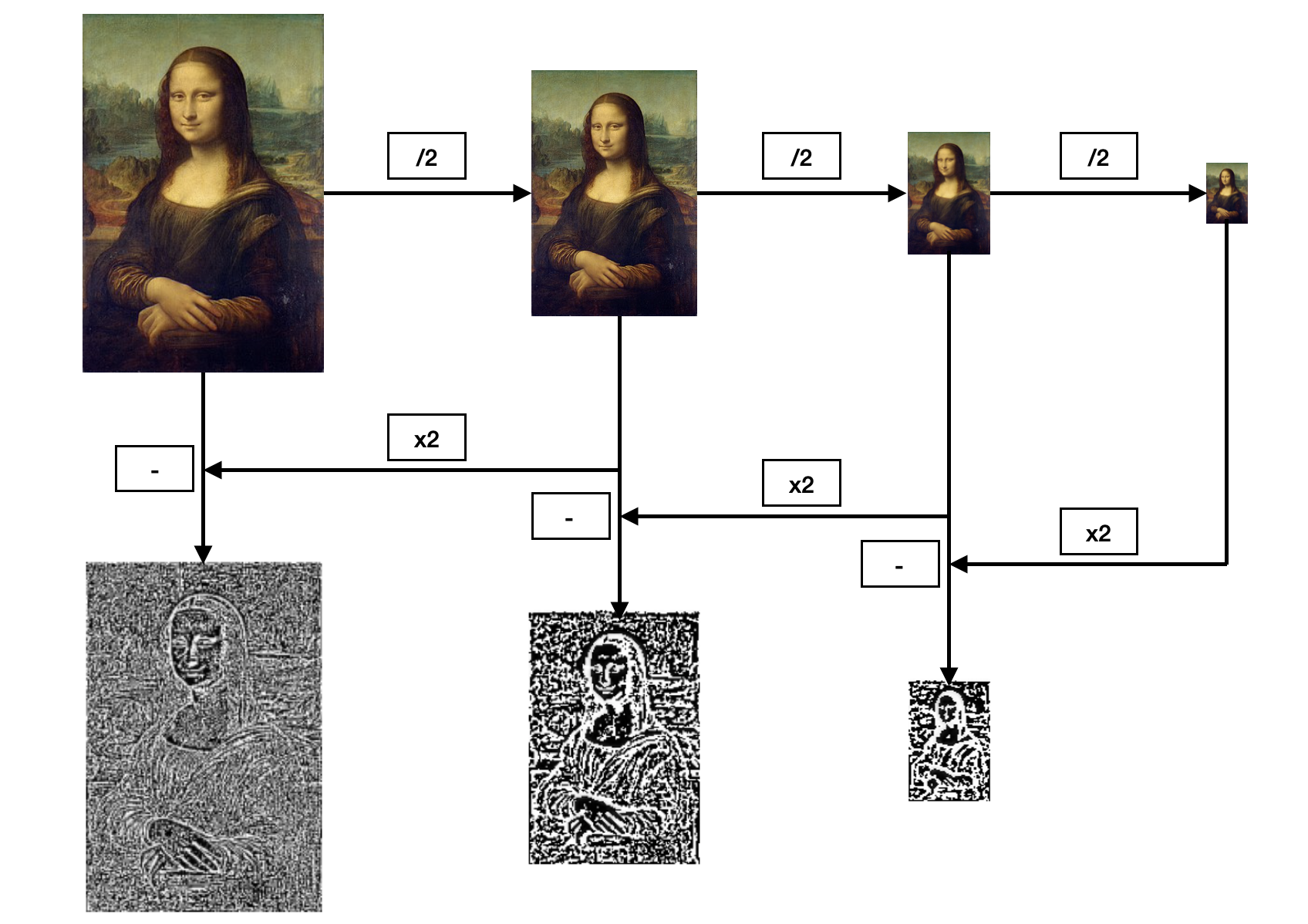
Laplacian Pyramid Construction with \(l = 3\)
For the next steps we will use all the levels of the Laplacian Pyramid.
Butterworth Filter
For the filtering step of the motions magnification, we want a filter that is tolerant to the frequencies outside of the given range as motions changes are not as uniform as colors changes. We will use a first order Butterworth Bandpass Filter as in [1].
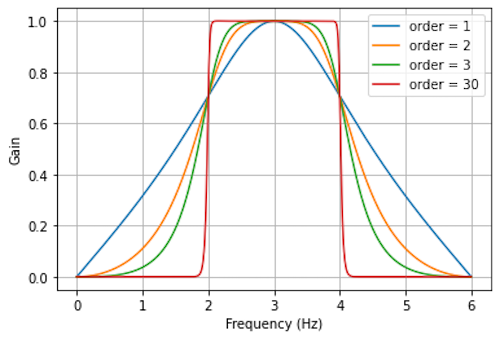
Butterworth Filter with \(\omega_{l} = 2\) and \(\omega_{h} = 4\)
In practice, to filter the images we start by computing the feedforward coefficient \(b_{i}\) and the feedback coefficient \(a_{i}\) of the Butterworth filter giving \([\omega_{l}, \omega_{h}]\) as the frequency range and the frame rate of the video as the signal sampling frequency. We then use this equation:
$$y[n] = \frac{1}{a_0}(b_{0}x[n] + b_{1}x[n - 1] - a_{1}y[n - 1])$$
Where \(y[n]\) is the \(n^{th}\) filtered Laplacian Pyramid and \(x[n]\) the \(n^{th}\) Laplacian Pyramid.
Note that \(y[0]\) and \(x[0]\) are equal to the Laplacian Pyramid of the first frame of the video.
Image Magnification & Reconstruction
Due to the fact that we are using all the levels of the Laplacian Pyramid, the magnification and reconstruction phase for the motions magnification is a little bit more complicated. First we need to dynamically adapt the amplification factor for each levels of the pyramid. To do so, we introduce the spatial wavelength \(\lambda\) representing a given level of the filtered Laplacian Pyramid \(F_{p}\). In our implementation \(\lambda\) is defined as follow:
$$\lambda = \sqrt{h^{2} + w^{2}}$$
Where \(h\) and \(w\) are respectively the height and the width of the considered \(F_{p}\) level. Moreover, \(\lambda\) and the amplification factor \(\alpha\) are linked by the following equation:
$$(1 + \alpha)\delta(t) < \frac{\lambda}{8}$$
Where \(\delta(t)\) is the displacement factor (see [1] for more details). We can now introduce the cutoff spatial wavelength \(\lambda_{c}\). With \(\lambda_{c}\), we can rewrite the previous equation as follow:
$$(1 + \alpha)\delta(t) = \frac{\lambda_{c}}{8} \implies \delta(t) = \frac{\frac{\lambda_{c}}{8}}{1 + \alpha}$$
The potentially new amplification factor \(\alpha_{new}\) for a given \(F_{p}\) level can be obtained with:
$$\alpha_{new} = \frac{\frac{\lambda}{8}}{\delta(t)} - 1$$
We obtain our amplification factor for a given \(F_{p}\) level \(l\) with:
$$\alpha_{l} = min(\alpha, \alpha_{new})$$
Similarly to the Gaussian Pyramid magnification, we obtain our magnified filtered pyramid level \(M_{F_{p}}[l]\) with attenuated chrominance with the following formula:
$$M_{F_{p}}[l] = \begin{cases}\alpha_{l} F_{p}[l]\ \text{if Y component}\\ \alpha_{l} A F_{p}[l]\ \text{if I or Q component}\end{cases}$$
We repeat the previous process for all the levels (except the first and last one) of \(F_{p}\).
Finally, we reconstruct our image by upsampling all the levels of \(M_{F_{p}}\) to the dimensions of the original image, adding it to the YIQ version of the original image, converting the resulting image to RGB and limiting the values of the resulting RGB image to \([0, 255]\) for each components. We repeat the previous process for each frame of the video.
Results
The code has been written in Python and it can be found on my github. Below you can see some results with the original video on the left side and the magnified one on the right side:
Colors Magnification
\(l = 4; \alpha = 50; A = 1; \omega_{l} = 0.8333; \omega_{h} = 1\)
\(l = 6; \alpha = 50; A = 1; \omega_{l} = 0.8333; \omega_{h} = 1\)
Motions Magnification
\(l = 4; \alpha = 15; \lambda_{c} = 16; A = 0.1; \omega_{l} = 0.4; \omega_{h} = 3\)
\(l = 6; \alpha = 30; \lambda_{c} = 16; A = 0.1; \omega_{l} = 0.4; \omega_{h} = 3\)
References
[1] Eulerian Video Magnification for Revealing Subtle Changes in the World by Hao-Yu Wu, Michael Rubinstein, Eugene Shih, John Guttag, Frédo Durand and William Freeman
[2] Fourier Transform by Robert Fisher, Simon Perkins, Ashley Walker and Erik Wolfart