Introduction
Image colorization is a two century old subject which was first tackled by photographers. As early as 1839, european photographers would hand-color monochrome photographs with a mixture of pigments and gum arabic. Although it emerged in Europe, the practice of image colorization gained tremendous popularity in Japan in the 1860s as it began to be considered as a refined art.
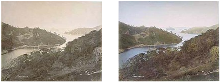
Monochrome photo (left) and Hand-colored version (right) by the Japan Photographic Association (1876-1885)
In the past century, dyes, watercolors, oils, crayons and pastels have also been used to colorize photographs but none really revolutionized the practice. The creation of computers and the emergence of softwares for image editing that followed initiated a change in the way the image colorization was done. The first to introduce computerized colorization was the Canadian engineer Wilson Markle in the 1970s. His method consisted of assigning predetermined colors to shades of gray in each scene. Nowadays, we see the emergence of deep learning based approaches that allow the automatic colorization of grayscale images. At first, the researchers used CNN and it gave pretty robust results as in [1]. We now see more and more approches based on Generative Adversarial Networks (GAN) and more specifically Deep Convolutional Generative Adversarial Networks (DCGAN) as in [2]. Here, we are going to present a DCGAN approach to the image colorization problem.
Pre-processing
The pre-processing phase consist of three different operations: resizing, color space conversion from RGB to LAB and normalization. The resizing will be performed to have either 32x32 or 256x256 images depending on the use case. The color space conversion from RGB to LAB is performed in order to better approximate the human perception between colors. And, the normalization is performed to make sure that we have values in the range \([-1, 1]\) for the model training. But what is the LAB color space and why do we have to use it instead of RGB ?
In order to quantify how similar or how different two colors are, we need a metric in the space of colors. LAB color space was historically designed so that the Euclidean distance between the coordinates of any colors in this space approximates as precisely as possible the human perception of distances between colors. That kind of color space is called perceptually uniform color space. We can, of course, apply the Euclidean distance to the RGB color space but the distance between two colors will not necessarily be higher if the colors are drastically different because RGB is not perceptually uniform.
The LAB color space is composed of three axis: the luminance/lightness (L) which is the grayscale axis, the red/green axis (a) and the yellow/blue axis (b). While L is in the range \([0, 100]\), a and b are in the range \([-128, 127]\).
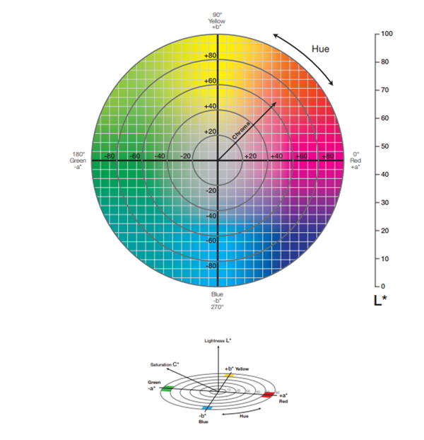
LAB color space chart
Moreover, due to the difference of ranges between the three channels of the LAB color space and in order to make sure that the values of the LAB image are in the good range for the training (i.e. \([-1, 1]\)), we have to divide the L channels by 100 and the a and b channels by 128. To learn more on the LAB color space and the conversion from RGB to LAB take a look at this site.
Model
As we are going to train a GAN, we will need two models: the generator and the discriminator. We are going to use the same architectures as in [2]. Thus, the generator will be a UNet-like model and the discriminator a simple CNN with 4 down-sampling layers similar to the contractive path of the generator.
![Architecture used for the generator in [2]](/static/colorization/architecture2.png)
Architecture used for the generator in [2]
However, we made a small change in the output of the generator. Instead of outputting the three LAB channels we output only the a and b channels as in [1].
Loss
In a traditional GAN, the input of the generator is a randomly generated noise. However, in our case the generator takes a grayscale image as input instead of noise. Since no noise is introduced, the input of the generator is treated as zero noise with the grayscale image as a prior. The discriminator will get colored images from both the generator and the original data and will try to tell which image has been generated and which image is the original one. This is what is called a Conditional Generative Adversarial Network.
In a formal way, the cost functions with L1 Regularization are defined as follow:
$$\min_{\theta_{G}} J^{(G)}(\theta_{D}, \theta_{G}) = \min_{\theta_{G}} -\mathop{\mathbb{E}}_{z}[log(D(G(0_{z}|x))] + \lambda || G(0_{z}|x) -y ||_{1}$$
$$\max_{\theta_{D}} J^{(D)}(\theta_{D}, \theta_{G}) = \max_{\theta_{D}}(\mathop{\mathbb{E}}_{y}[log(D(y|x))]+ \mathop{\mathbb{E}}_{z}[log(1 - D(G(0_{z}|x)|x))])$$
In practice, we can define them as follow:
$$G_{loss} = BCELoss(G(x), 1) + \lambda \cdot L1Loss(G(x), y)$$
$$D_{loss} = BCELoss(D(y), 1) + BCELoss(D(G(x)), 0)$$
Where \(1\) is the “real” label, \(0\) is the “fake” label, \(x\) the grayscale input image and \(y\) the a and b channels of the orignal image in the LAB color space.
Post-processing
The post-processing consist of three simple steps. First, we retrieve the output of the model, which are the predicted a and b channels, and we stack the input grayscale image on top of this output. We then multiply the L channel by 100 and the a and b channels by 128 in order to obtain a proper LAB image. Finally we convert the LAB image to RGB.
Configuration & Results
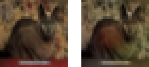
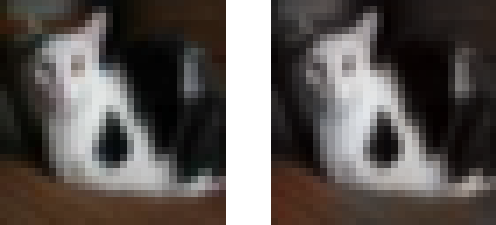
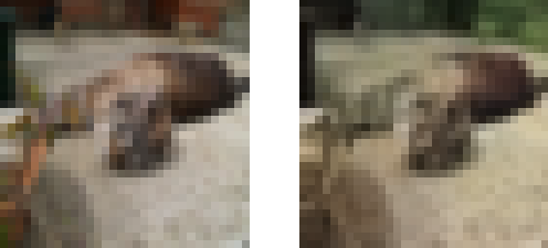
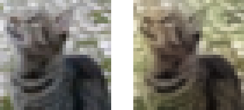
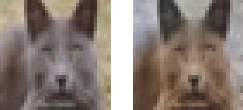
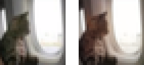
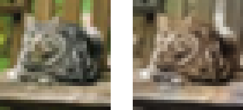
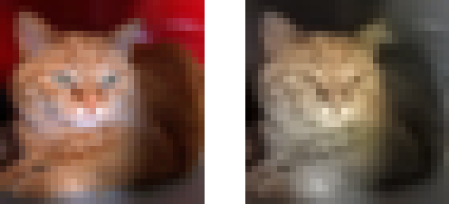
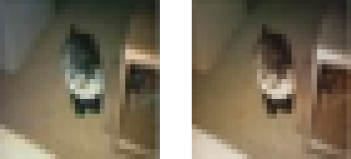
The model has been trained using a Kaggle GPU Notebook with the CIFAR-10 Dataset[3]. We splitted the data into 80% for training, 10% for validation and 10% for testing. We used almost the same configuration as in [2]: a batch size of 128; Adam optimizer with a learning rate of 0.0002, a \(\beta_{1}\) of 0.5 and a \(\beta_{2}\) of 0.999; a \(\lambda\) of 100 and an early stopping patience of 5. We launched the training for 200 epochs and it stopped, due to the early stopping patience, at the epoch 19. The code has been written in Python and Pytorch and it can be found on my github. Note that, due to the lack of VRAM, we used FP32 precision (float) instead of FP64 precision (double) that is present in the code. Below you can see some of the results on the testing set with the original 32x32 image on the left and the colorized 32x32 image on the right:
References
[1] Colorful Image Colorization by Richard Zhang, Philip Isola and Alexei A. Efros
[2] Image Colorization using Generative Adversarial Networks by Kamyar Nazeri, Eric Ng and Mehran Ebrahimi
[3] CIFAR-10 Dataset